CBSE Class 12 › Unit III: Magnetic Effects

Moving Charges & Magnetism

NCERT Chapter 4 • Full Notes, Derivations & Diagrams

NCERT 2025–26 Unit III • ~8 Marks JEE Main • 2-3 Questions

1. Magnetic Force (Lorentz Force)

Oersted discovered that moving charges or currents produce a magnetic field. The force on a charge $q$ moving with velocity $\vec{v}$ in a magnetic field $\vec{B}$ and electric field $\vec{E}$ is given by the Lorentz Force.

\vec{F} = q[\vec{E} + (\vec{v} \times \vec{B})]

Magnetic Force: $\vec{F}_m = q(\vec{v} \times \vec{B})$

Right-hand rule diagram showing the relationship between velocity, magnetic field, and magnetic force. — The magnetic force acts perpendicular to both velocity and magnetic field.

Key Features of Magnetic Force:

It depends on $q, v$ and $B$ . Force is zero if charge is at rest ( $v=0$ ).
It is zero if $\vec{v}$ is parallel or antiparallel to $\vec{B}$ ( $\sin 0^\circ = 0$ ).
It acts perpendicular to $\vec{v}$ , so no work is done by the magnetic force. Kinetic energy and speed remain constant.

Force on Current Carrying Conductor
For a rod of length $l$ carrying current $I$ :

\vec{F} = I(\vec{l} \times \vec{B})

2. Motion in a Magnetic Field

Since the magnetic force is perpendicular to velocity, it acts as a centripetal force, causing the particle to undergo circular or helical motion.

Helical path of a charged particle moving at an angle to a magnetic field. — When velocity has a component parallel to B, the path becomes a helix.

Case 1: $\vec{v} \perp \vec{B}$ (Circular Motion)
The magnetic force provides centripetal force: $qvB = \dfrac{mv^2}{r}$ .

Radius: $r = \dfrac{mv}{qB}$
Frequency (Cyclotron Frequency): $\nu = \dfrac{qB}{2\pi m}$ (Independent of speed!)

Case 2: $\vec{v}$ at angle $\theta$ to $\vec{B}$ (Helical Motion)
Velocity has two components: $v_{\perp} = v \sin\theta$ (circular motion) and $v_{\parallel} = v \cos\theta$ (linear motion).

Pitch (p): Distance moved along B in one rotation. $p = v_{\parallel} T = \dfrac{2\pi m v \cos\theta}{qB}$

3. Biot-Savart Law

This law gives the magnetic field produced by a current element $I d\vec{l}$ .

d\vec{B} = \dfrac{\mu_0}{4\pi} \dfrac{I d\vec{l} \times \vec{r}}{r^3}

Magnitude: $dB = \dfrac{\mu_0}{4\pi} \dfrac{I dl \sin\theta}{r^2}$

Where $\mu_0 = 4\pi \times 10^{-7} \, \text{T m/A}$ is the permeability of free space.

4. Derivation: Field on Axis of Circular Loop

Consider a circular loop of radius $R$ carrying current $I$ . We wish to find the field at point P on the axis at distance $x$ .

Diagram showing geometry for calculating magnetic field on the axis of a circular current loop. — Components perpendicular to the axis cancel out; only axial components sum up.

Derivation: Field on Axis 5 Marks

Step 1: Field due to element dl
The distance $r$ from element to P is $r = \sqrt{x^2 + R^2}$ .
Since $dl \perp r$ , the magnitude is $dB = \dfrac{\mu_0}{4\pi} \dfrac{I dl}{r^2}$ .

Step 2: Resolving Components
$dB$ has an axial component $dB_x = dB \cos\theta$ and a perpendicular component $dB_{\perp} = dB \sin\theta$ .
By symmetry, $\sum dB_{\perp} = 0$ . Only $dB_x$ survives.

Step 3: Geometry Factors
From the figure, $\cos\theta = \dfrac{R}{r} = \dfrac{R}{(x^2 + R^2)^{1/2}}$ .

Step 4: Integration
Total Field $B = \int dB_x = \int \dfrac{\mu_0 I dl}{4\pi r^2} \cdot \dfrac{R}{r}$ .
Since $r$ is constant for the loop, $\int dl = 2\pi R$ (Circumference).

Step 5: Final Result
$B = \dfrac{\mu_0 I R}{4\pi r^3} (2\pi R) = \dfrac{\mu_0 I R^2}{2(x^2 + R^2)^{3/2}}$ .
At centre ( $x=0$ ): $B = \dfrac{\mu_0 I}{2R}$ .

5. Ampere’s Circuital Law

The line integral of magnetic field $\vec{B}$ around any closed loop is equal to $\mu_0$ times the net current $I$ threading through the loop.

\oint \vec{B} \cdot d\vec{l} = \mu_0 I_{enclosed}

Application: Field of a Solenoid

Cross-section of a solenoid with an Amperian loop for deriving magnetic field. — Using Ampere’s Law on a rectangular loop ABCD to find the field inside a solenoid.

Derivation: Field inside Long Solenoid 3 Marks

Step 1: Amperian Loop
Consider a rectangular loop of length $h$ . Field inside is parallel to axis; field outside is approx zero.

Step 2: Line Integral
$\oint \vec{B} \cdot d\vec{l} = Bh + 0 + 0 + 0 = Bh$ . (Sides perpendicular to B give 0, outside is 0).

Step 3: Enclosed Current
If $n$ is turns per unit length, total turns in length $h$ is $nh$ . Total current $I_e = I (nh)$ .

Step 4: Result
$Bh = \mu_0 (nh I) \Rightarrow$ $B = \mu_0 n I$ .

6. Force Between Two Parallel Currents

Two parallel wires carrying currents exert magnetic force on each other. This phenomenon is used to define the SI unit “Ampere”.

Diagram illustrating magnetic force between two parallel current-carrying conductors. — Parallel currents attract; antiparallel currents repel.

Derivation: Force per unit length 3 Marks

Step 1: Field produced by Wire A
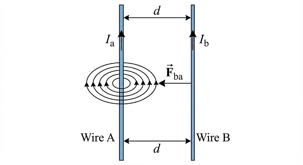
Field at distance $d$ due to current $I_a$ : $B_a = \dfrac{\mu_0 I_a}{2\pi d}$ .

Step 2: Force on Wire B
Wire B carries $I_b$ in field $B_a$ . Force on length $L$ :
$F_{ba} = I_b L B_a = I_b L \left( \dfrac{\mu_0 I_a}{2\pi d} \right)$ .

Step 3: Force per unit length
$f = \dfrac{F}{L} = \dfrac{\mu_0 I_a I_b}{2\pi d}$ .

Definition of Ampere: One ampere is that steady current which, when maintained in two very long, parallel conductors 1m apart in vacuum, produces a force of $2 \times 10^{-7}$ N per metre of length.

7. Torque on Current Loop & Magnetic Dipole

A rectangular loop carrying current $I$ placed in a uniform magnetic field $\vec{B}$ does not experience a net force, but it experiences a torque. This behavior is analogous to an electric dipole in an electric field.

Diagram showing forces acting on a rectangular current loop in a magnetic field. — Forces on the arms form a couple, creating torque that rotates the coil.

Derivation: Torque on a Rectangular Loop 5 Marks

Step 1: Setup
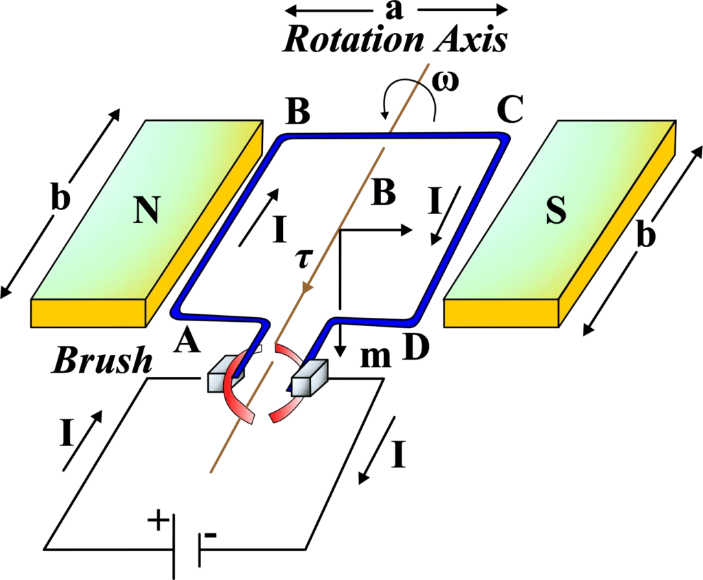
Consider a rectangular loop of sides $a$ and $b$ , carrying current $I$ . Area $A = ab$ .
The loop is placed in a uniform magnetic field $B$ . Let the normal to the area of the coil make an angle $\theta$ with the field $\vec{B}$ .

Step 2: Forces on the Arms

Arms BC and DA (length $a$ ): The forces on these arms are equal and opposite and act along the same axis (the axis of the coil). They cancel each other out, resulting in no net torque from these sides.
Arms AB and CD (length $b$ ): These arms are perpendicular to $\vec{B}$ . The force on each arm is $F = I b B$ .

Step 3: Calculating Torque
The forces $F$ on arms AB and CD are equal, opposite, and act along different lines of action. They form a couple.
The perpendicular distance (lever arm) between these two forces is $a \sin \theta$ .
Torque $\tau = \text{Force} \times \text{Lever Arm}$ .

Step 4: Substitution
$\tau = (IbB) \times (a \sin \theta)$
Rearranging terms: $\tau = I (ab) B \sin \theta$ .
Since $A = ab$ (Area of the loop):
$\tau = I A B \sin \theta$ .

Step 5: For N turns
If the coil has $N$ closely wound turns, the torque increases by a factor of $N$ :
$\tau = N I A B \sin \theta$ .

Magnetic Dipole Moment

The magnetic moment ( $\vec{m}$ ) of a current loop is defined as the product of the current and the area vector.

\vec{m} = N I \vec{A}

\vec{\tau} = \vec{m} \times \vec{B}

Direction of $\vec{m}$ is given by Right-Hand Thumb Rule.

Analogy with Electrostatics:
The current loop behaves like a magnetic dipole.

Electric Dipole: $\vec{\tau} = \vec{p} \times \vec{E}$
Magnetic Dipole: $\vec{\tau} = \vec{m} \times \vec{B}$

Equilibrium:

Stable: $\theta = 0^\circ$ ( $\vec{m} \parallel \vec{B}$ ). Torque is zero.
Unstable: $\theta = 180^\circ$ ( $\vec{m}$ antiparallel to $\vec{B}$ ). Torque is zero.

8. Moving Coil Galvanometer

A sensitive instrument to detect currents. It uses a radial magnetic field to ensure the torque is maximum and constant at any deflection.

Construction of a moving coil galvanometer showing radial field and soft iron core. — The radial magnetic field ensures constant torque at all angles.

Principle:
Magnetic torque = Restoring torque of spring.
$N I A B = k \phi$
Where $\phi$ is deflection and $k$ is torsional constant.

1. Current Sensitivity:
Deflection per unit current: $\dfrac{\phi}{I} = \dfrac{NAB}{k}$ .

2. Voltage Sensitivity:
Deflection per unit voltage: $\dfrac{\phi}{V} = \dfrac{NAB}{kR}$ .

Conversion:

To Ammeter: Connect a low resistance (shunt) in parallel.
To Voltmeter: Connect a high resistance in series.

← Previous: Current Electricity Next: Magnetism & Matter →