AP Physics 1 Kinematics: The "Big 4" Equations & Formulas (2026 Guide)

Figure 1.1. Constant-acceleration motion showing the five variables used throughout AP Physics 1 kinematics.

Master the four constant-acceleration equations used throughout AP Physics 1. Learn what each equation means, when to apply it, and how to solve one-dimensional motion problems using the notation adopted in AP Physics.

📘 AP Physics 1 📖 Unit 1: Kinematics 🎯 College Board Aligned ⭐ Beginner Friendly

AP Exam Tip

The Big 4 kinematics equations are valid only for motion with constant acceleration. Before choosing an equation, always verify that the acceleration remains constant throughout the motion.

Quick Summary

Kinematics is the study of how objects move without considering the forces that cause the motion. In AP Physics 1, nearly every one-dimensional motion problem with constant acceleration can be solved using the Big 4 Kinematics Equations.

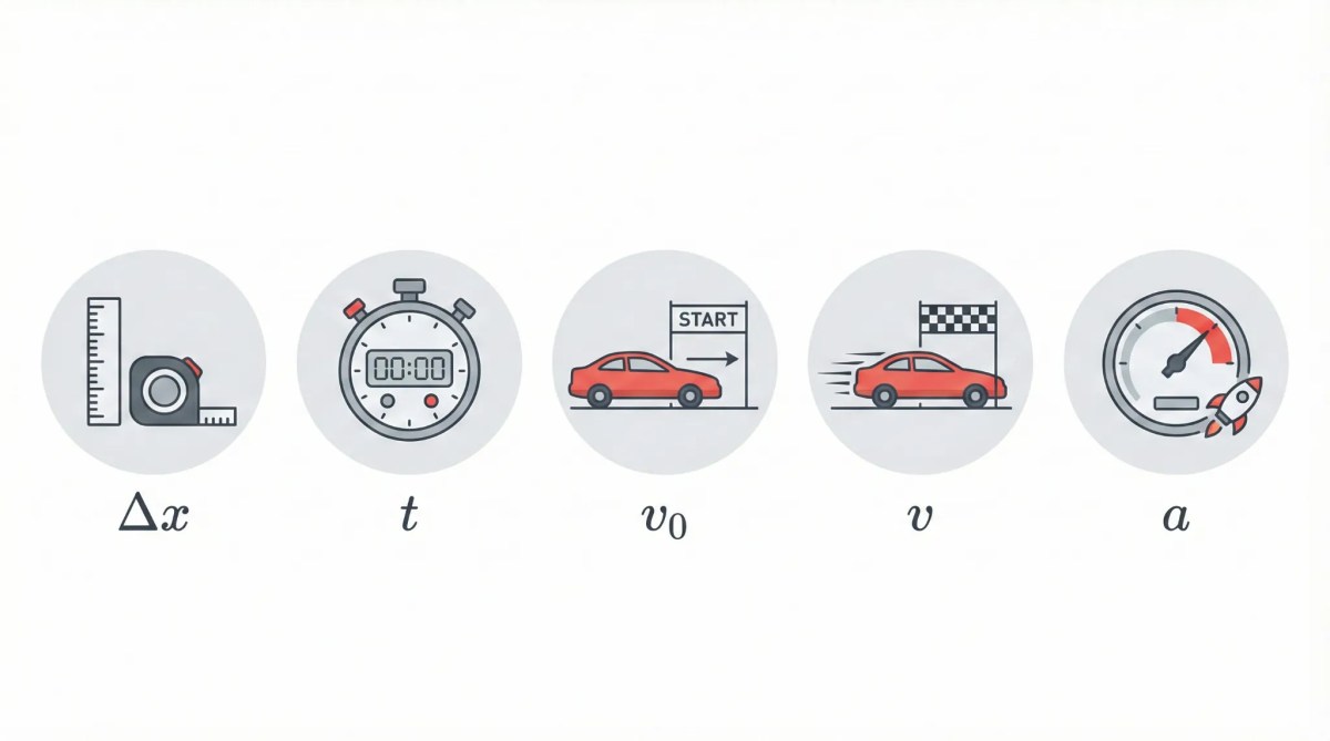
Every problem is built around five motion variables:

Initial velocity $v_0$
Final velocity $v$
Displacement $\Delta x$
Acceleration $a$
Time $t$

The key to solving any kinematics problem is identifying which variables are known, determining the unknown quantity, and selecting the equation that contains the required variables.

Overview of AP Physics kinematics showing displacement, velocity, acceleration, time, and the Big 4 equations — **Figure 2.1.** Kinematics connects the five motion variables using four constant-acceleration equations.

What You’ll Learn

By the end of this lesson, you will be able to:

Identify Motion Variables

Recognize the five variables used in constant-acceleration motion and understand their physical meaning.

Select the Correct Equation

Determine which kinematics equation to use based on the known and unknown variables.

Solve AP-Style Problems

Apply the Big 4 equations to horizontal motion, free-fall motion, and typical AP Physics exam questions.

Avoid Common Mistakes

Recognize frequent calculation and sign-convention errors before they cost you points on the AP exam.

Why This Lesson Matters

The Big 4 kinematics equations are among the most frequently used equations in AP Physics 1. They are the foundation for later topics such as projectile motion, Newton’s laws, circular motion, and energy. A strong understanding of these equations will make nearly every mechanics chapter easier to learn.

What Is Kinematics?

Kinematics is the branch of mechanics that studies how objects move without considering the forces responsible for that motion. Instead of asking why an object moves, kinematics focuses on describing the motion using measurable quantities such as position, displacement, velocity, acceleration, and time.

Throughout AP Physics 1, most one-dimensional motion problems assume that the object moves with constant acceleration. Under this condition, the relationships between the motion variables can be described using the Big 4 Kinematics Equations.

AP Physics diagram illustrating straight-line motion with displacement, velocity, acceleration, and time — **Figure 3.1.** Kinematics describes motion using measurable quantities without considering the forces that produce the motion.

Think About It

Imagine watching a car travel along a straight highway. Even if you know nothing about the engine or the force produced by the tires, you can still answer questions such as:

How far did the car travel?
How fast is it moving?
How long did the trip take?
Is the car speeding up or slowing down?

These are all kinematics questions because they describe the object’s motion without explaining what caused it.

The Five Variables of Motion

Every constant-acceleration problem in AP Physics 1 involves five measurable quantities. Before selecting a kinematics equation, identify which variables are known and which variable you need to determine.

Symbol	Quantity	SI Unit	Description
$v_0$	Initial Velocity	m/s	The velocity of the object at the beginning of its motion.
$v$	Final Velocity	m/s	The velocity after a given time or displacement.
$\Delta x$	Displacement	m	The change in position of the object.
$a$	Acceleration	m/s²	The rate at which velocity changes with time.
$t$	Time	s	The duration of the motion.

Five variables used in AP Physics kinematics: initial velocity, final velocity, displacement, acceleration, and time — **Figure 3.2.** Every constant-acceleration problem can be solved using combinations of these five variables.

Common Mistake

Do not confuse distance with displacement. Distance measures the total path travelled, whereas displacement measures the straight-line change in position from the starting point to the ending point. The Big 4 equations always use $\Delta x$ , not distance.

Concept Check

A runner completes one full lap around a 400 m circular track and finishes at the starting point.

What is the runner’s displacement?

Show Answer

The displacement is $0\,\text{m}$ because the runner’s final position is the same as the starting position, even though the total distance travelled is 400 m.

The Big 4 Kinematics Equations

The four kinematics equations describe the relationship between initial velocity $v_0$ , final velocity $v$ , displacement $\Delta x$ , acceleration $a$ , and time $t$ for motion with constant acceleration.

Each equation connects a different combination of these five variables. Rather than memorizing them randomly, learn which variable each equation leaves out. This makes choosing the correct equation much easier during problem solving.

Overview of the four AP Physics kinematics equations and the variables they connect — **Figure 4.1.** The Big 4 Kinematics Equations relate the five variables of motion in different ways.

How to use equations — **Figure 4.2.** Which equation to use when.

Before Using Any Equation

✔ Motion must have constant acceleration.
✔ Write the known variables.
✔ Identify the unknown quantity.
✔ Choose the equation that contains only one unknown.

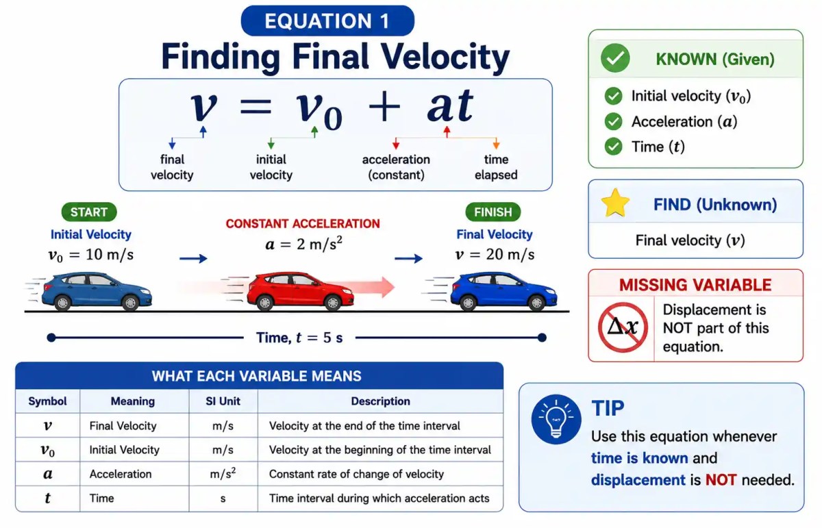
Equation 1: Finding Final Velocity

The first kinematics equation relates initial velocity, acceleration, time, and final velocity. It is the simplest of the four equations and is often the first equation students use in AP Physics 1.

Use this equation whenever you know the object’s initial velocity, acceleration, and the time interval, and you need to determine its final velocity.

Visual explanation of the first kinematics equation showing a car accelerating from initial velocity to final velocity — **Figure 5.1.** Equation 1 predicts how an object’s velocity changes with time when acceleration remains constant.

The Equation

$v=v_0+at$

What Each Variable Means

Symbol	Meaning	SI Unit
$v$	Final Velocity	m/s
$v_0$	Initial Velocity	m/s
$a$	Acceleration	m/s²
$t$	Time	s

When Should You Use This Equation?

✔ Acceleration is constant.
✔ Time is known.
✔ Displacement is not required.
✔ You need the final velocity.

Remember

This equation does not contain displacement $\Delta x$ . If displacement is part of the unknown information, choose a different kinematics equation.

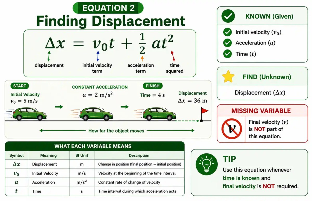
Equation 2: Finding Displacement

The second kinematics equation determines an object’s displacement when its initial velocity, constant acceleration, and elapsed time are known. Unlike Equation 1, this equation predicts how far the object moves during the given time interval.

Use this equation whenever you know $v_0$ , $a$ , and $t$ , and you need to calculate the displacement $\Delta x$ .

Visual explanation of the second kinematics equation showing displacement, initial velocity, acceleration, and time — **Figure 6.1.** Equation 2 calculates displacement using initial velocity, acceleration, and elapsed time.

The Equation

$\Delta x=v_0t+\frac12at^2$

What Each Variable Means

Symbol	Meaning	SI Unit
$\Delta x$	Displacement	m
$v_0$	Initial Velocity	m/s
$a$	Acceleration	m/s²
$t$	Time	s

When Should You Use This Equation?

✔ Motion has constant acceleration.
✔ Initial velocity is known.
✔ Time is known.
✔ You need displacement.
✔ Final velocity is NOT known.

Remember

This equation does not include the final velocity $v$ . If the final velocity is known, Equation 4 may be a better choice.

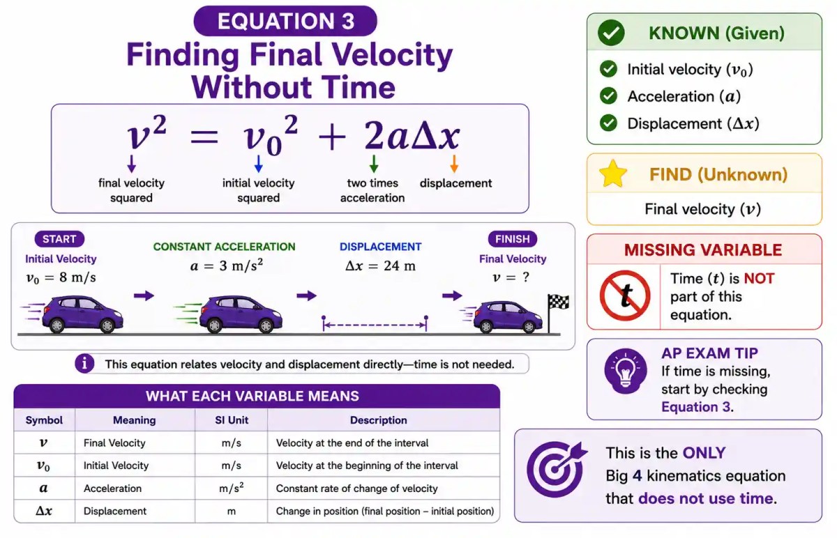
Equation 3: Finding Final Velocity Without Time

The third kinematics equation is unique because it allows you to calculate the final velocity without knowing the time taken. Instead, it relates initial velocity, acceleration, and displacement.

Whenever time is unknown—or not required—this equation is usually the best choice.

Visual explanation of the third kinematics equation showing final velocity without using time — **Figure 7.1.** Equation 3 relates velocity, displacement, and acceleration without using time.

The Equation

$v^2=v_0^2+2a\Delta x$

What Each Variable Means

Symbol	Meaning	SI Unit
$v$	Final Velocity	m/s
$v_0$	Initial Velocity	m/s
$a$	Acceleration	m/s²
$\Delta x$	Displacement	m

When Should You Use This Equation?

✔ Motion has constant acceleration.
✔ Time is unknown.
✔ Initial velocity is known.
✔ Displacement is known.
✔ You need the final velocity.

Remember

This is the only Big 4 kinematics equation that does not contain time. If time is missing from the problem, check this equation first.

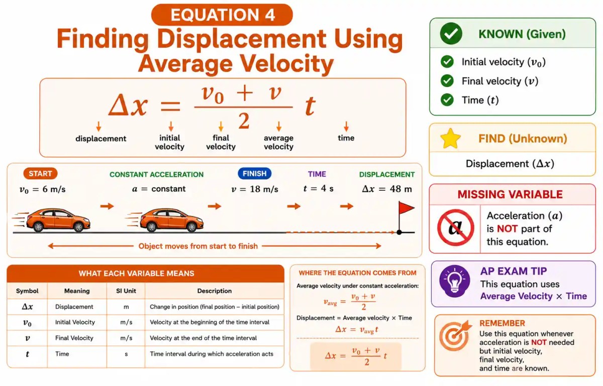
Equation 4: Finding Displacement Using Average Velocity

The fourth kinematics equation calculates an object’s displacement by multiplying its average velocity by the elapsed time. When acceleration is constant, the average velocity is simply the average of the initial and final velocities.

Use this equation whenever you know the initial velocity, final velocity, and time, and you need to determine the displacement.

Visual explanation of the fourth kinematics equation showing displacement from average velocity — **Figure 8.1.** Equation 4 calculates displacement using average velocity during constant acceleration.

The Equation

$\Delta x=\frac{v_0+v}{2}t$

What Each Variable Means

Symbol	Meaning	SI Unit
$\Delta x$	Displacement	m
$v_0$	Initial Velocity	m/s
$v$	Final Velocity	m/s
$t$	Time	s

When Should You Use This Equation?

✔ Motion has constant acceleration.
✔ Initial velocity is known.
✔ Final velocity is known.
✔ Time is known.
✔ You need displacement.

Remember

This equation does not include acceleration $a$ . If acceleration is unknown but the initial velocity, final velocity, and time are available, this equation is often the fastest solution.

Comparing the Big 4 Kinematics Equations

One of the easiest ways to select the correct kinematics equation is to identify which variable is missing. Each of the Big 4 equations leaves out exactly one of the five motion variables.

Instead of memorizing four separate formulas, remember which variable each equation does not contain.

Comparison chart showing the four AP Physics kinematics equations, their uses, and missing variables — **Figure 9.1.** Each kinematics equation omits one variable. Choose the equation that excludes the unknown quantity.

Equation	Use It To Find	Missing Variable	Best Used When
$v=v_0+at$	Final Velocity	$\Delta x$	Time is known and displacement is not needed.
$\Delta x=v_0t+\frac12at^2$	Displacement	$v$	Final velocity is unknown.
$v^2=v_0^2+2a\Delta x$	Final Velocity	$t$	Time is unknown.
$\Delta x=\frac{v_0+v}{2}t$	Displacement	$a$	Acceleration is unknown.

Quick Rule

Identify the quantity you don’t know. Then choose the equation that does not contain that missing variable.

Concept Check

You know $v_0$ , $a$ , and $\Delta x$ , but the time is unknown. Which equation should you choose?

Show Answer

Use $v^2=v_0^2+2a\Delta x$ because it is the only equation that does not contain time.

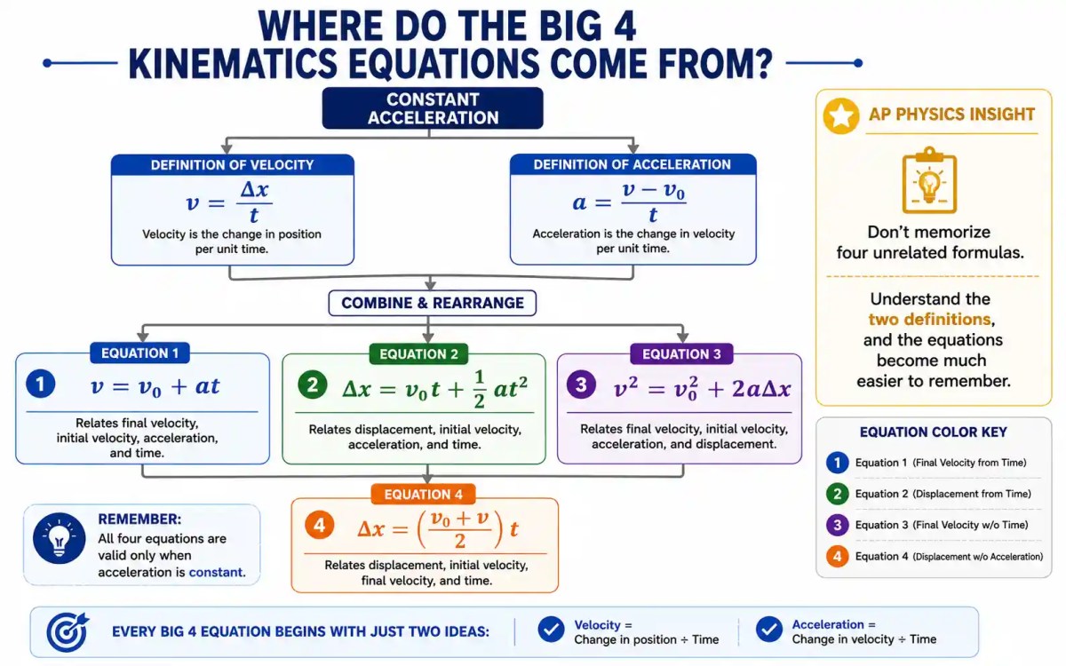
Where Do the Big 4 Kinematics Equations Come From?

The Big 4 kinematics equations are not independent formulas. They are all derived from two fundamental ideas: the definition of velocity and the definition of acceleration. Assuming acceleration remains constant, these definitions can be combined to produce every equation you’ve learned.

Understanding the derivations helps you remember the equations more naturally and gives you confidence when solving unfamiliar problems.

Flowchart showing how the four kinematics equations are derived from the definitions of velocity and acceleration — **Figure 10.1.** All four kinematics equations originate from the definitions of velocity and acceleration under constant acceleration.

Key Idea

You only need two basic definitions to derive every kinematics equation. The remaining formulas are mathematical consequences of those definitions.

Derivation of Equation 1

The first kinematics equation is obtained directly from the definition of constant acceleration. By rearranging the acceleration equation, we can express the final velocity in terms of the initial velocity, acceleration, and elapsed time.

Step-by-step derivation of the first kinematics equation using the definition of acceleration — **Figure 11.1.** Deriving the first kinematics equation from the definition of constant acceleration.

Step 1: Start with the Definition of Acceleration

$a=\frac{v-v_0}{t}$

Acceleration is the rate at which velocity changes with time.

Step 2: Multiply Both Sides by Time

$at=v-v_0$

Step 3: Add $v_0$ to Both Sides

$v=v_0+at$

Final Result

$\boxed{v=v_0+at}$

What Does This Equation Tell Us?

The final velocity equals the initial velocity plus the change in velocity produced by constant acceleration over time.

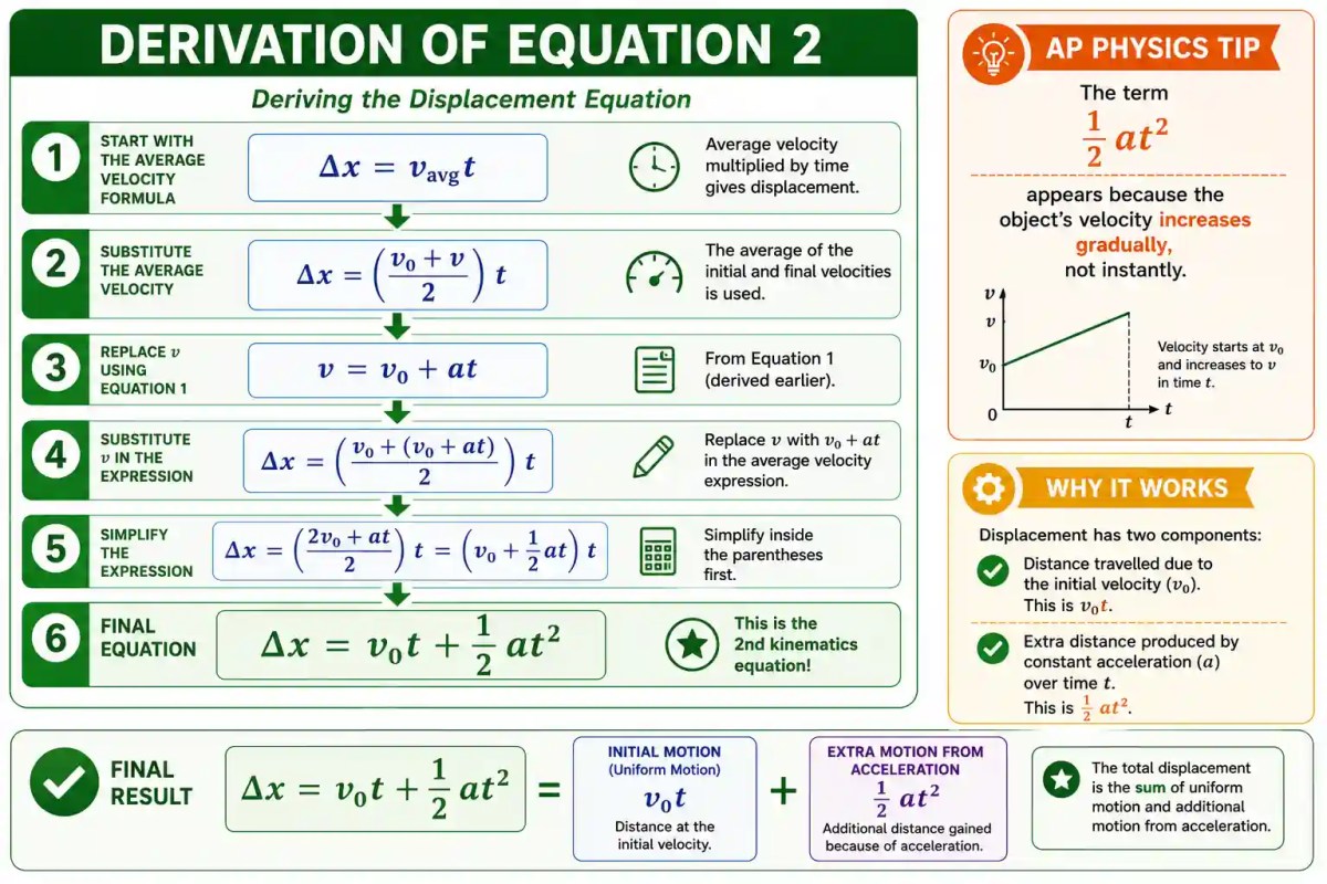
Derivation of Equation 2

The second kinematics equation is obtained by combining the definition of average velocity with the first kinematics equation. This derivation shows why the displacement depends on both the object’s initial velocity and the additional distance covered due to constant acceleration.

Step-by-step derivation of the second kinematics equation from average velocity and constant acceleration — **Figure 12.1.** Deriving the second kinematics equation using average velocity and constant acceleration.

Step 1: Start with the Average Velocity Formula

$\Delta x=v_{\text{avg}}t$

Step 2: Substitute the Average Velocity

$\Delta x=\frac{v_0+v}{2}t$

Step 3: Replace $v$ Using Equation 1

$v=v_0+at$

$\Delta x=\frac{v_0+(v_0+at)}{2}t$

Step 4: Simplify

$\Delta x=v_0t+\frac12at^2$

Final Result

$\boxed{\Delta x=v_0t+\frac12at^2}$

Physical Meaning

The displacement consists of two parts: the distance covered at the initial velocity $(v_0t)$ and the additional distance caused by constant acceleration $\left(\frac12at^2\right)$ .

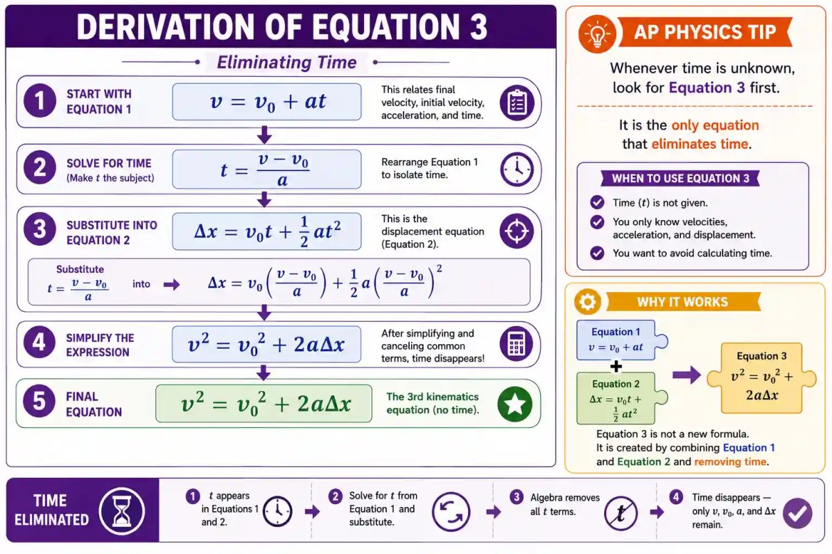
Derivation of Equation 3

The third kinematics equation is obtained by eliminating time from the first two equations. Instead of introducing a new idea, it combines equations you already know to relate velocity, acceleration, and displacement directly.

Step-by-step derivation of the third kinematics equation by eliminating time — **Figure 13.1.** Deriving the third kinematics equation by eliminating time from Equations 1 and 2.

Step 1: Start with Equation 1

$v=v_0+at$

Step 2: Rearrange to Make Time the Subject

$t=\frac{v-v_0}{a}$

Step 3: Substitute into Equation 2

$\Delta x=v_0t+\frac12at^2$

Substitute the expression for $t$ from Step 2 into the displacement equation.

Step 4: Simplify the Algebra

$v^2=v_0^2+2a\Delta x$

Final Result

$\boxed{v^2=v_0^2+2a\Delta x}$

What Makes This Equation Special?

This is the only Big 4 kinematics equation that does not contain time. It is especially useful when the elapsed time is unknown or unnecessary.

Derivation of Equation 4

The fourth kinematics equation comes directly from the definition of average velocity. When acceleration is constant, the average velocity is simply the average of the initial and final velocities. Multiplying this average velocity by time gives the total displacement.

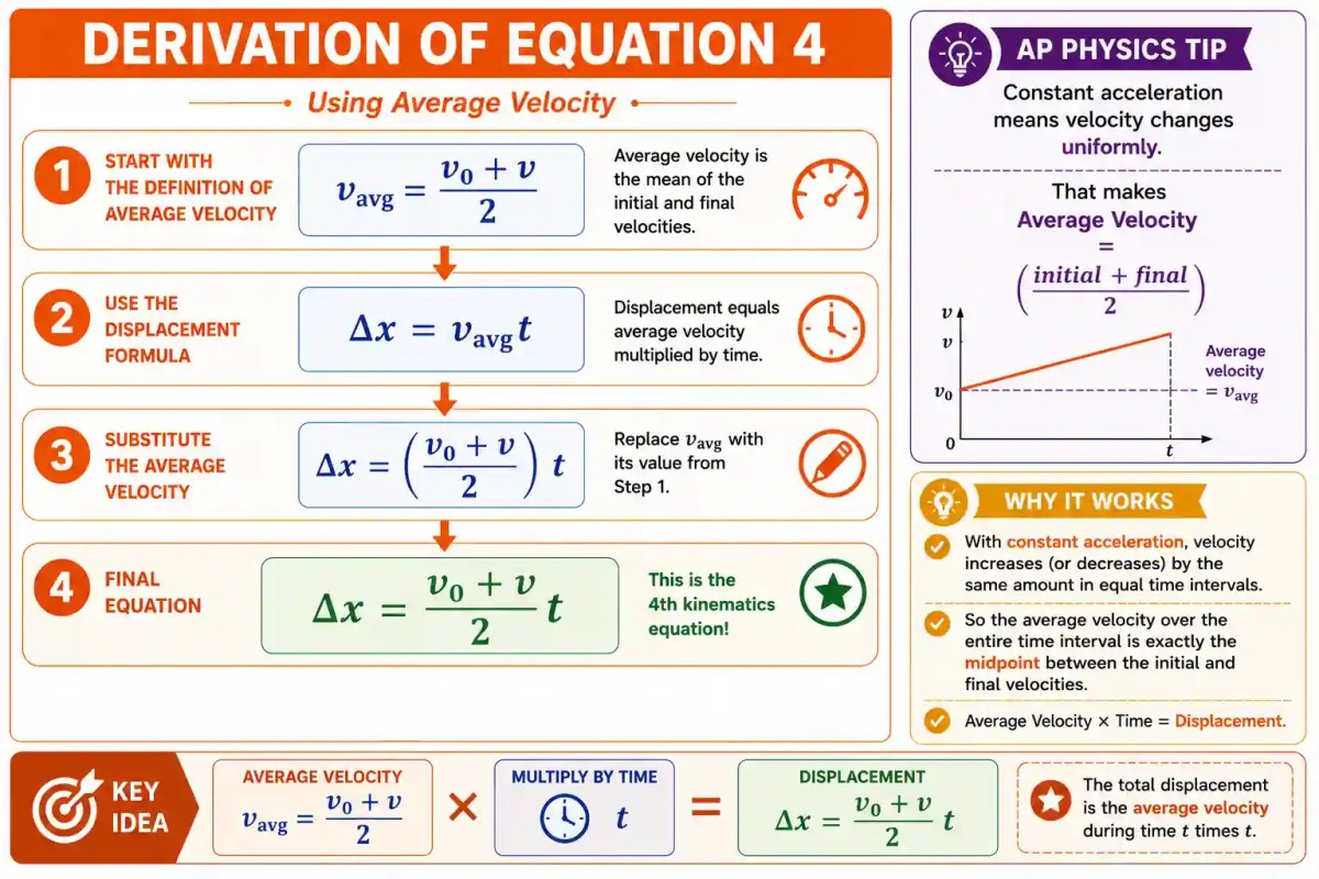
Step-by-step derivation of the fourth kinematics equation using average velocity — **Figure 14.1.** Deriving the fourth kinematics equation from the definition of average velocity.

Step 1: Start with the Definition of Average Velocity

$v_{\text{avg}}=\frac{v_0+v}{2}$

Step 2: Use the Displacement Formula

$\Delta x=v_{\text{avg}}t$

Step 3: Substitute the Average Velocity

$\Delta x=\left(\frac{v_0+v}{2}\right)t$

Final Result

$\boxed{\Delta x=\frac{v_0+v}{2}t}$

Why This Equation Works

With constant acceleration, velocity changes uniformly over time. Therefore, the average velocity is simply the midpoint between the initial and final velocities. Multiplying that average velocity by time gives the displacement.

How to Choose the Correct Kinematics Equation

One of the biggest challenges in AP Physics is deciding which equation to use. Instead of memorizing all four formulas, identify the variables you know, determine the quantity you need to find, and eliminate equations that contain additional unknowns.

The flowchart below provides a quick decision-making strategy that works for almost every constant-acceleration problem.

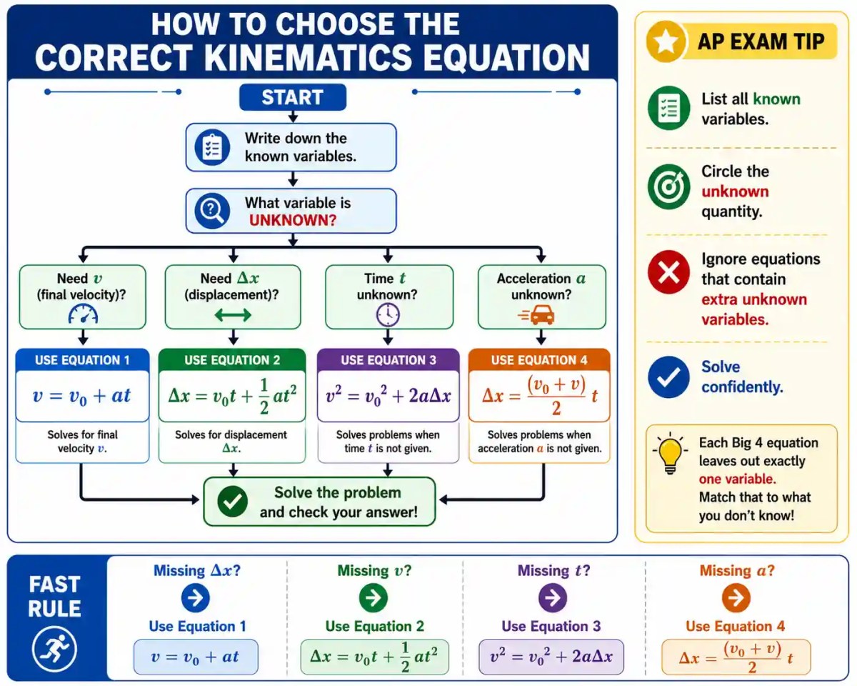
Flowchart showing how to choose the correct kinematics equation — **Figure 15.1.** A simple decision tree for selecting the correct AP Physics kinematics equation.

Three-Step Strategy

Write down every known variable.
Circle the unknown quantity.
Select the equation that contains only one unknown.

Remember

Each Big 4 equation leaves out exactly one variable. If that missing variable matches the quantity you don’t know, you’ve probably found the correct equation.

Common Mistake

Students often choose an equation because it looks familiar. Instead, choose the equation based on the variables provided in the problem.

Worked Example 1: Finding the Final Velocity

A car starts from rest and accelerates uniformly at 3.0 m/s² for 8.0 seconds. What is its final velocity?

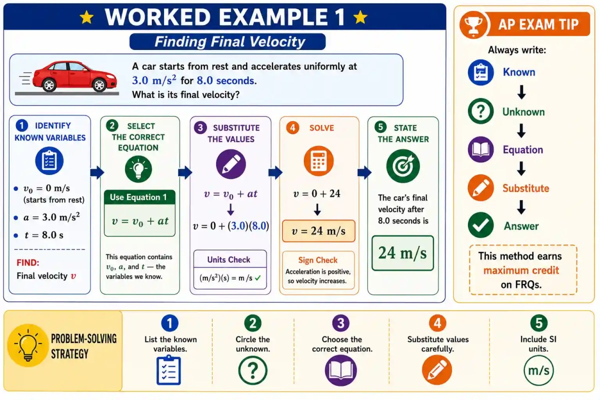
Worked example calculating final velocity using the first kinematics equation — **Figure 16.1.** Using Equation 1 to calculate the final velocity of an accelerating car.

Step 1: Identify the Known Variables

$v_0=0\text{ m/s}$
$a=3.0\text{ m/s}^2$
$t=8.0\text{ s}$
Find $v$

Step 2: Select the Correct Equation

$v=v_0+at$

Step 3: Substitute the Values

$v=0+(3.0)(8.0)$

Step 4: Solve

$v=24\text{ m/s}$

Answer

The car’s final velocity after 8.0 seconds is

$\boxed{24\text{ m/s}}$

Why Equation 1?

The displacement is not needed in this problem. Since the known variables are the initial velocity, acceleration, and time, Equation 1 is the most direct choice.

Worked Example 2: Finding Displacement

A cyclist is moving at an initial velocity of 5.0 m/s and accelerates uniformly at 2.0 m/s² for 6.0 seconds. How far does the cyclist travel during this time?

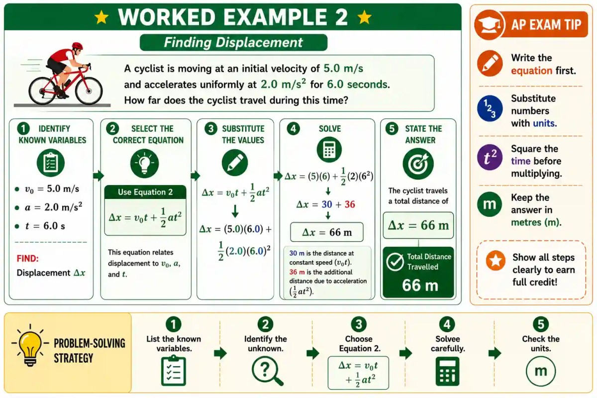
Worked example calculating displacement using the second kinematics equation — **Figure 17.1.** Using Equation 2 to calculate displacement during constant acceleration.

Step 1: Identify the Known Variables

$v_0 = 5.0\ \text{m/s}$
$a = 2.0\ \text{m/s}^2$
$t = 6.0\ \text{s}$
Find $\Delta x$

Step 2: Select the Correct Equation

$\Delta x = v_0t+\frac12at^2$

Step 3: Substitute the Values

$\Delta x=(5.0)(6.0)+\frac12(2.0)(6.0)^2$

Step 4: Solve

$\Delta x=30+36=66\text{ m}$

Answer

$\boxed{\Delta x=66\text{ m}}$

Why Equation 2?

The final velocity is not given and is not required. Equation 2 directly relates displacement to the known quantities: initial velocity, acceleration, and time.

Worked Example 3: Finding Final Velocity Without Time

A runner starts at an initial velocity of 4.0 m/s and accelerates uniformly at 3.0 m/s² over a displacement of 20 m. What is the runner’s final velocity?

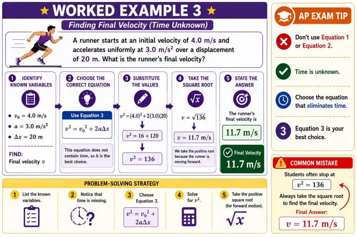
Worked example calculating final velocity without knowing time using Equation 3 — **Figure 18.1.** Using Equation 3 when time is unknown.

Step 1: Identify the Known Variables

$v_0 = 4.0\ \text{m/s}$
$a = 3.0\ \text{m/s}^2$
$\Delta x = 20\ \text{m}$
Find $v$

Step 2: Choose the Correct Equation

$v^2=v_0^2+2a\Delta x$

Notice that this equation does not contain time, making it the ideal choice.

Step 3: Substitute the Values

$v^2=(4.0)^2+2(3.0)(20)$

$v^2=16+120=136$

Step 4: Take the Square Root

$v=\sqrt{136}=11.7\text{ m/s}$

Answer

$\boxed{v\approx11.7\text{ m/s}}$

Why Equation 3?

Time is not given and is not required. Equation 3 directly relates velocity, acceleration, and displacement, making it the most efficient choice.

Worked Example 4: Finding Displacement Using Average Velocity

A train increases its speed uniformly from 12.0 m/s to 28.0 m/s in 8.0 seconds. How far does the train travel during this time?

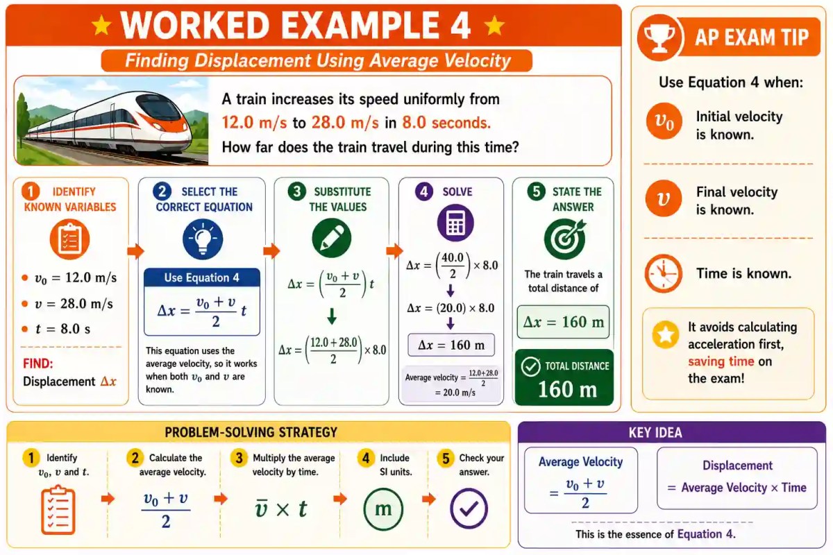
Worked example calculating displacement using average velocity — **Figure 19.1.** Using Equation 4 to calculate displacement from average velocity.

Step 1: Identify the Known Variables

$v_0 = 12.0\ \text{m/s}$
$v = 28.0\ \text{m/s}$
$t = 8.0\ \text{s}$
Find $\Delta x$

Step 2: Select the Correct Equation

$\Delta x=\frac{v_0+v}{2}t$

Step 3: Substitute the Values

$\Delta x=\frac{12.0+28.0}{2}\times8.0$

Step 4: Solve

$\Delta x=20.0\times8.0=160\text{ m}$

Answer

$\boxed{\Delta x=160\text{ m}}$

Why Equation 4?

Both the initial and final velocities are known. Under constant acceleration, the average velocity is simply the average of these two values, making Equation 4 the quickest solution.

Applying the Big 4 Equations to Free Fall

The four kinematics equations are not limited to horizontal motion. They also describe free fall, including objects that are dropped, thrown upward, or projected downward, provided the acceleration remains constant. In free fall, the constant acceleration is due to gravity.

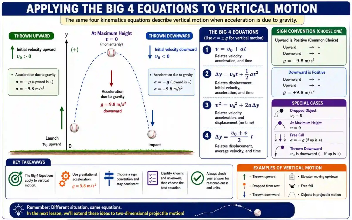
Using the Big 4 kinematics equations for vertical motion under gravity — **Figure 20.1.** The Big 4 equations apply to free fall by replacing acceleration with gravitational acceleration.

Gravity Acts as Constant Acceleration

In AP Physics, the variable $g$ represents the magnitude of gravitational acceleration (approximately $9.8m/s^2$ ). Whether it is written as $+g$ or $−g$ depends entirely on the coordinate system you choose.

When air resistance is neglected, every freely moving object near Earth’s surface accelerates downward at approximately

$g = 9.8\ \text{m/s}^2$

If upward is chosen as the positive direction, then

$a=-g=-9.8\ \text{m/s}^2$

If downward is chosen as positive, then

$a=+9.8\ \text{m/s}^2$

Choose one sign convention and use it consistently throughout the entire problem.

The Same Four Equations Still Apply

Horizontal Motion	Vertical Motion
$a=\text{constant}$	$a=\pm g$
$\Delta x$	$\Delta y$
$v_0$	$v_0$
$v$	$v$
$t$	$t$

Special Cases to Remember

Dropped object: $v_0=0$
Maximum height: $v=0$
Free fall: acceleration is always due to gravity.
Thrown downward: the initial velocity is directed downward.

Quick Reference: Solving Free-Fall Problems

Use this checklist before solving any free-fall or vertical-motion problem.

✔ Dropped object: $v_0 = 0$
✔ At maximum height: $v = 0$
✔ If upward is positive: $a = -9.8\ \text{m/s}^2$
✔ If downward is positive: $a = +9.8\ \text{m/s}^2$
✔ Apply the same Big 4 kinematics equations.

Worked Example: Finding Maximum Height

A ball is thrown vertically upward with an initial velocity of 20.0 m/s. Assuming air resistance is negligible, determine the maximum height reached by the ball.

Step 1: Identify the Variables

$v_0=20.0\text{ m/s}$
$v=0\text{ m/s}$
$a=-9.8\text{ m/s}^2$
Find $\Delta y$

Step 2: Select the Equation

$v^2=v_0^2+2a\Delta y$

Step 3: Substitute the Values

$0=(20.0)^2+2(-9.8)\Delta y$

$0=400-19.6\Delta y$

$\Delta y=\frac{400}{19.6}=20.4\text{ m}$

Answer

$\boxed{\Delta y=20.4\text{ m}}$

Common Mistakes

Using the wrong sign for gravitational acceleration.
Forgetting that the velocity is zero only at the highest point.
Changing the positive direction halfway through the solution.
Using distance instead of displacement.

AP Exam Tip

Whenever a problem involves an object moving upward or downward, don’t memorize new equations. Simply apply the same Big 4 equations using the correct sign for gravitational acceleration.

Mixed AP Physics Practice Problems

Now it’s your turn. In the following problems, you are not told which equation to use. Start by identifying the known variables, determine the unknown quantity, and then choose the most appropriate kinematics equation.

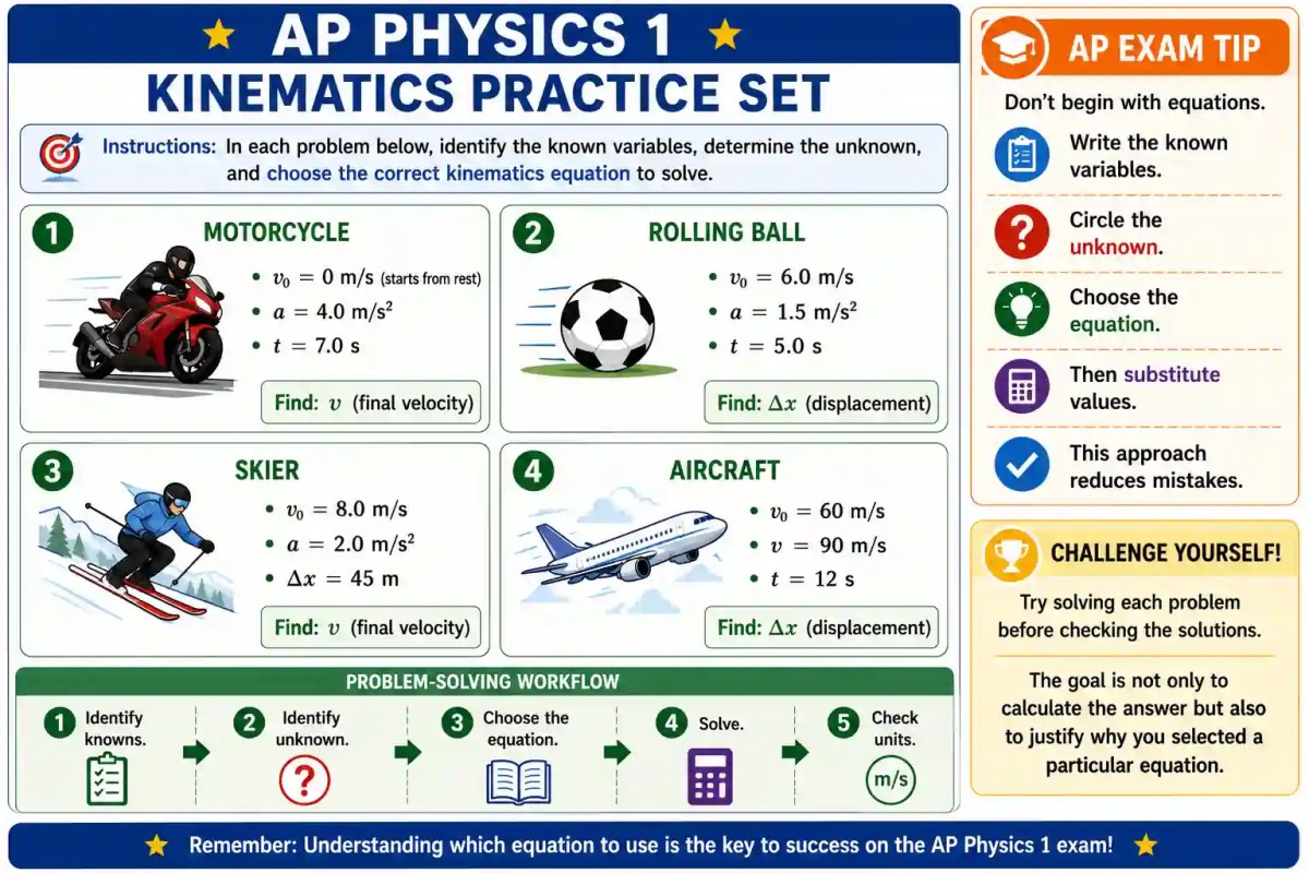
AP Physics kinematics practice problems worksheet — **Figure 21.1.** Four mixed AP Physics practice problems covering all Big 4 equations.

Problem 1

A motorcycle starts from rest and accelerates at 4.0 m/s² for 7.0 s. Determine its final velocity.

Problem 2

A ball rolls with an initial velocity of 6.0 m/s and accelerates at 1.5 m/s² for 5.0 s. How far does it travel?

Problem 3

A skier moves 45 m while accelerating uniformly at 2.0 m/s². If the initial velocity is 8.0 m/s, find the final velocity.

Problem 4

An aircraft increases its speed from 60 m/s to 90 m/s in 12 s. Determine the displacement.

Challenge Yourself

Try solving each problem before checking the solutions. The goal is not only to calculate the answer but also to justify why you selected a particular equation.

Solutions to the Practice Problems

Check your work using the solutions below. Compare not only your final answer but also the equation you selected. Choosing the correct equation is just as important as performing the calculations correctly.

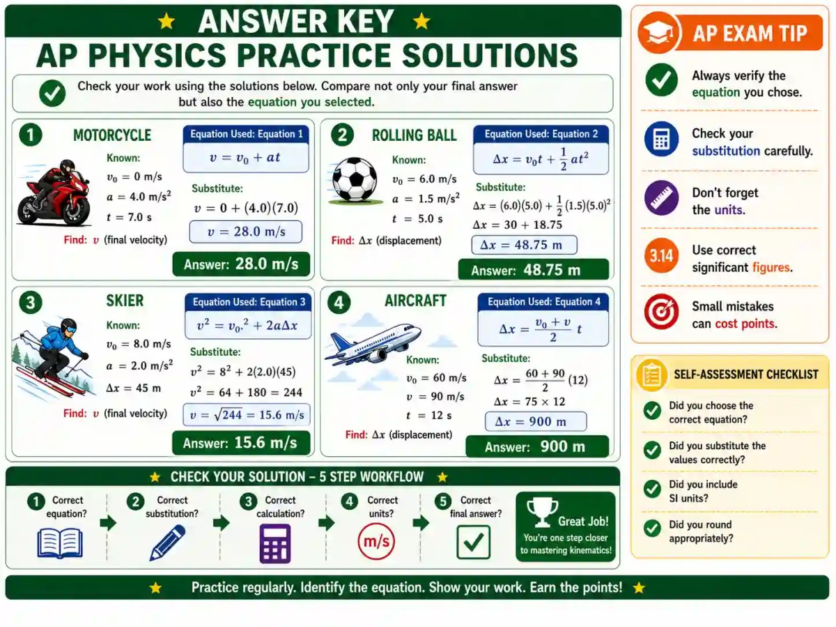
Answer key for AP Physics kinematics practice problems — **Figure 22.1.** Solutions to the mixed AP Physics practice problems.

Problem 1

Equation Used:

$v=v_0+at$

$v=0+(4.0)(7.0)=28.0\text{ m/s}$

Answer: 28.0 m/s

Problem 2

$\Delta x=v_0t+\frac12at^2$

$\Delta x=(6.0)(5.0)+\frac12(1.5)(5.0)^2$

$\Delta x=30+18.75=48.75\text{ m}$

Answer: 48.75 m

Problem 3

$v^2=v_0^2+2a\Delta x$

$v^2=8^2+2(2)(45)=244$

$v=\sqrt{244}=15.6\text{ m/s}$

Answer: 15.6 m/s

Problem 4

$\Delta x=\frac{v_0+v}{2}t$

$\Delta x=\frac{60+90}{2}(12)=900\text{ m}$

Answer: 900 m

Self-Assessment

✔ Did you choose the correct equation?
✔ Did you substitute the values correctly?
✔ Did you include SI units?
✔ Did you round appropriately?

Common Kinematics Mistakes (Avoid These Errors!)

Many mistakes in AP Physics are not caused by difficult mathematics—they happen because students rush, choose the wrong equation, or forget basic problem-solving steps. Reviewing these common errors can help you avoid losing easy marks.

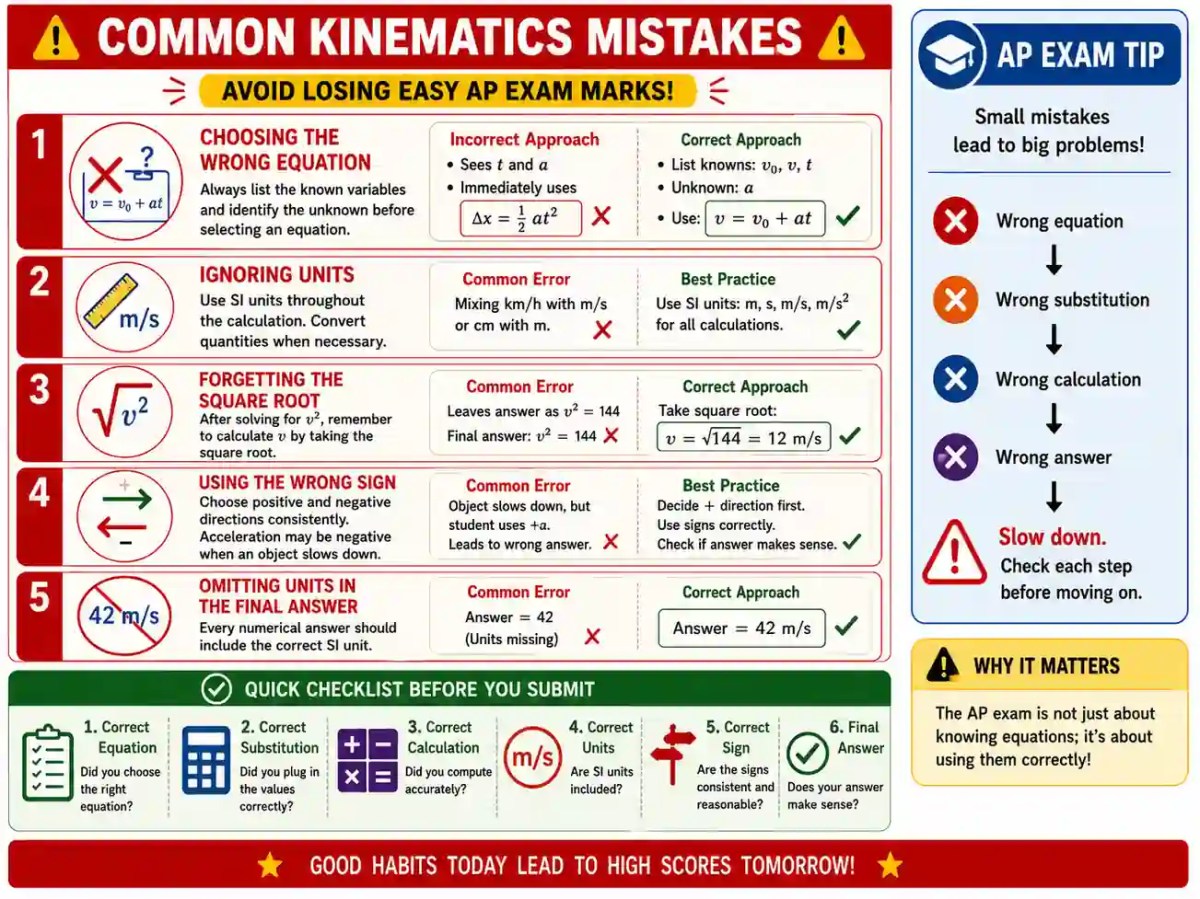
Common mistakes when solving AP Physics kinematics problems — **Figure 23.1.** Common mistakes students make when solving constant-acceleration problems.

1. Choosing the Wrong Equation

Always list the known variables and identify the unknown before selecting an equation.

2. Ignoring Units

Use SI units throughout the calculation. Convert quantities when necessary.

3. Forgetting the Square Root

After solving for $v^2$ , remember to calculate $v$ by taking the square root.

4. Using the Wrong Sign

Choose positive and negative directions consistently. Acceleration may be negative when an object slows down.

5. Omitting Units in the Final Answer

Every numerical answer should include the correct SI unit, such as m, m/s, or m/s².

Quick Checklist Before You Submit

✔ Correct equation selected
✔ Values substituted correctly
✔ Units included
✔ Correct sign used
✔ Final answer checked

AP Physics Exam Strategy for Kinematics

Success in AP Physics depends on more than knowing the equations. High-scoring students follow a consistent problem-solving strategy that helps them avoid mistakes and earn maximum credit on both multiple-choice and free-response questions.

AP Physics kinematics exam strategy infographic — **Figure 24.1.** A proven workflow for solving kinematics problems efficiently on the AP Physics exam.

Five-Step Exam Strategy

Read the entire question before writing anything.
List all known variables and identify the unknown.
Select the kinematics equation with only one unknown.
Show every substitution and calculation clearly.
Check units, signs, and whether the final answer is physically reasonable.

FRQ Scoring Advice

✔ Start with the equation before substituting numbers.
✔ Show every algebraic step.
✔ Include SI units throughout your work.
✔ Box or clearly indicate your final answer.

Don’t Lose Easy Marks

Many students lose points because they rush into calculations without identifying the correct equation. Spending a few seconds planning your approach often saves much more time later.

Big 4 Kinematics Cheat Sheet

Need a quick review? This cheat sheet summarizes the four constant-acceleration equations, when to use each one, and the variables involved. Save it for quick revision before quizzes, homework, or the AP Physics exam.

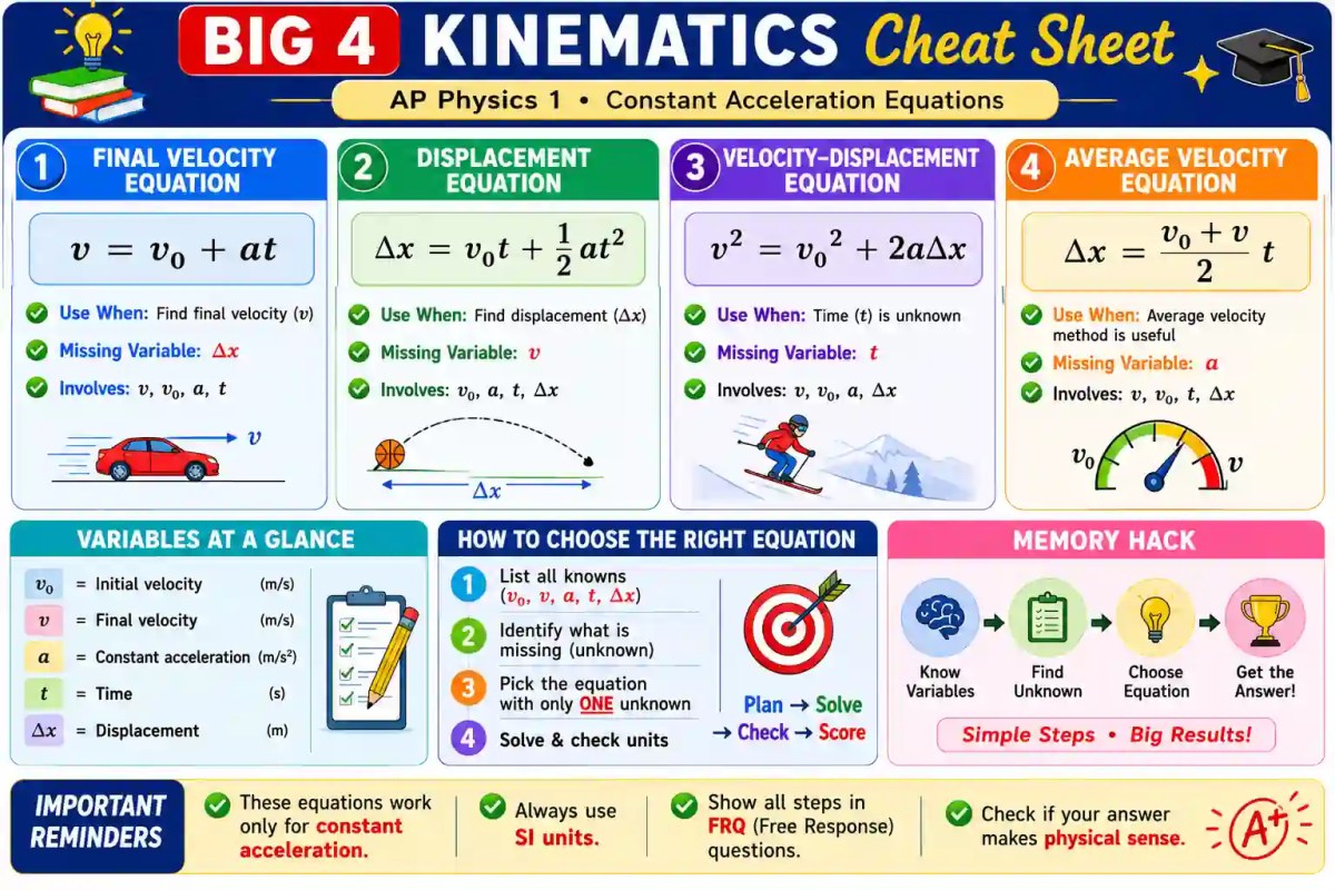
AP Physics Big 4 kinematics equations cheat sheet — **Figure 25.1.** A one-page reference for the Big 4 kinematics equations.

Equation	Use When	Missing Variable
$v=v_0+at$	Find final velocity	$\Delta x$
$\Delta x=v_0t+\frac12at^2$	Find displacement	$v$
$v^2=v_0^2+2a\Delta x$	Time is unknown	$t$
$\Delta x=\frac{v_0+v}{2}t$	Average velocity method	$a$

Variables

$v_0$ = Initial velocity
$v$ = Final velocity
$a$ = Constant acceleration
$t$ = Time
$\Delta x$ = Displacement

Quick Revision Tip

Before choosing an equation, identify which variable is missing. The correct equation is usually the one that contains all the known variables and only one unknown.

Frequently Asked Questions (FAQ)

Still have questions? These quick answers address some of the most common doubts students have when learning and applying the Big 4 kinematics equations in AP Physics 1.

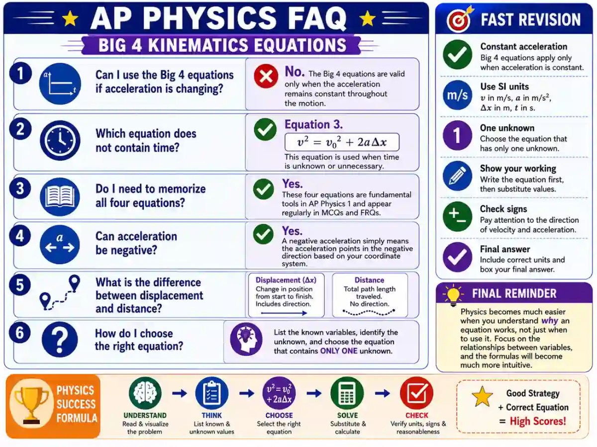
AP Physics kinematics frequently asked questions — **Figure 26.1.** Quick answers to common AP Physics kinematics questions.

Can I use the Big 4 equations if acceleration is changing?

No. The Big 4 equations are valid only when the acceleration remains constant throughout the motion.

How do I know which equation to use?

List the known variables, identify the unknown quantity, and choose the equation that contains only one unknown.

Do I need to memorize all four equations?

Yes. These equations are fundamental tools in AP Physics 1 and appear regularly in both multiple-choice and free-response questions.

What is the difference between displacement and distance?

Displacement measures the change in position and includes direction, while distance is the total path traveled.

Can acceleration be negative?

Yes. A negative acceleration simply means the acceleration points in the negative direction based on your chosen coordinate system.

Which equation does not contain time?

$v^2=v_0^2+2a\Delta x$

Equation 3 is used whenever time is unknown or unnecessary.

Final Reminder

Physics becomes much easier when you understand why an equation works, not just when to use it. Focus on the relationships between variables, and the formulas will become much more intuitive.

Lesson Summary & Next Steps

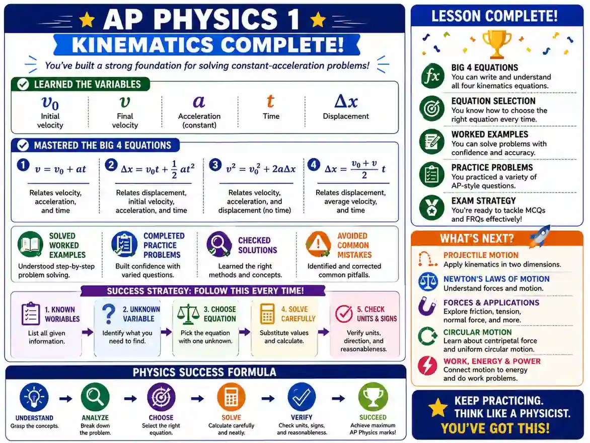
Congratulations! You have completed one of the most important topics in AP Physics 1. By understanding when and how to use the Big 4 kinematics equations, you have built a strong foundation for solving constant-acceleration problems with confidence.

Summary of the AP Physics kinematics equations lesson — **Figure 27.1.** The essential ideas to remember after studying the Big 4 kinematics equations.

Key Takeaways

✔ The Big 4 equations apply only when acceleration is constant.
✔ Always begin by identifying the known variables and the unknown quantity.
✔ Select the equation that contains only one unknown.
✔ Include SI units and check the direction (sign) of each quantity.
✔ Verify that your final answer is physically reasonable.

Keep Practicing

The best way to master kinematics is by solving a variety of problems. As you encounter new situations, focus on the relationships between variables rather than memorizing procedures. With practice, choosing the correct equation becomes almost automatic.

Continue Your AP Physics Journey

Once you’re comfortable with constant-acceleration motion, you’re ready to explore topics such as projectile motion, Newton’s laws of motion, forces, circular motion, and energy. Each builds on the problem-solving skills developed in this lesson.

Quick Summary

What You’ll Learn

Identify Motion Variables

Select the Correct Equation

Solve AP-Style Problems

Avoid Common Mistakes

Why This Lesson Matters

What Is Kinematics?

Think About It

The Five Variables of Motion

Common Mistake

Concept Check

The Big 4 Kinematics Equations

Before Using Any Equation

Equation 1: Finding Final Velocity

The Equation

What Each Variable Means

When Should You Use This Equation?

Remember

Equation 2: Finding Displacement

The Equation

What Each Variable Means

When Should You Use This Equation?

Remember

Equation 3: Finding Final Velocity Without Time

The Equation

What Each Variable Means

When Should You Use This Equation?

Remember

Equation 4: Finding Displacement Using Average Velocity

The Equation

What Each Variable Means

When Should You Use This Equation?

Remember

Comparing the Big 4 Kinematics Equations

Quick Rule

Concept Check

Where Do the Big 4 Kinematics Equations Come From?

Key Idea

Derivation of Equation 1

Step 1: Start with the Definition of Acceleration

Step 2: Multiply Both Sides by Time

Step 3: Add to Both Sides

Final Result

What Does This Equation Tell Us?

Derivation of Equation 2

Step 1: Start with the Average Velocity Formula

Step 2: Substitute the Average Velocity

Step 3: Replace Using Equation 1

Step 4: Simplify

Final Result

Physical Meaning

Derivation of Equation 3

Step 1: Start with Equation 1

Step 2: Rearrange to Make Time the Subject

Step 3: Substitute into Equation 2

Step 4: Simplify the Algebra

Final Result

What Makes This Equation Special?

Derivation of Equation 4

Step 1: Start with the Definition of Average Velocity

Step 2: Use the Displacement Formula

Step 3: Substitute the Average Velocity

Final Result

Why This Equation Works

How to Choose the Correct Kinematics Equation

Three-Step Strategy

Remember

Common Mistake

Worked Example 1: Finding the Final Velocity

Step 1: Identify the Known Variables

Step 2: Select the Correct Equation

Step 3: Substitute the Values

Step 4: Solve

Answer

Why Equation 1?

Worked Example 2: Finding Displacement

Step 1: Identify the Known Variables

Step 2: Select the Correct Equation

Step 3: Substitute the Values

Step 3: Add $v_0$ to Both Sides

Step 3: Replace $v$ Using Equation 1