CBSE Class 12 › Unit I: Electrostatics

Electric Charges & Fields

NCERT Class 12 Physics • Chapter 1 • Full Notes & Derivations

NCERT 2025–26 Unit I (Electrostatics) • ~9 Marks JEE Main • 1–2 Questions

Topic	Question Type	Marks (Approx.)
Field Lines / Properties	MCQ / Assertion	1
Dipole Fields (Axial & Equatorial)	Short Answer / Derivation	3
Gauss Law + Applications	Long Answer (Derivations)	5

1. Electric Charge & Coulomb’s Law

Electric charge is an intrinsic property of matter. Like charges repel, unlike charges attract. Benjamin Franklin introduced the convention of positive and negative charges.

Three Basic Properties of Charge

Additivity: Total charge is the scalar sum $q_{total} = q_1 + q_2 + \dots$ .
Conservation: Charge is neither created nor destroyed in an isolated system, only transferred.
Quantisation: $q = \pm ne$ , where $n$ is an integer and $e$ is elementary charge.

Quantisation of Charge

q = \pm ne

$e = 1.602 \times 10^{-19}\,\text{C}$

Coulomb’s Law

The electrostatic force between two stationary point charges is along the line joining them, directly proportional to the product of charges and inversely proportional to the square of the separation.

Vector Form

\vec{F}_{21} = \dfrac{1}{4\pi\epsilon_0} \dfrac{q_1 q_2}{r_{21}^2} \hat{r}_{21}

$k \approx 9 \times 10^9\,\text{N m}^2\text{C}^{-2}$

Vector diagram showing two point charges q1 and q2 separated by distance r, with repulsive force vectors F12 and F21 along the line joining them. — Vector representation of Coulomb’s Law for two like charges.

⚠️

Superposition Principle: Net force on a charge due to multiple charges is the vector sum of individual forces: $\vec{F}_{net} = \vec{F}_1 + \vec{F}_2 + \dots + \vec{F}_n$ .

2. Electric Field & Field Lines

The electric field at a point is defined as the force experienced by a unit positive test charge placed at that point, with the source charges undisturbed.

Field of a Point Charge

\vec{E} = \dfrac{1}{4\pi\epsilon_0} \dfrac{Q}{r^2} \hat{r}

Units: N/C or V/m

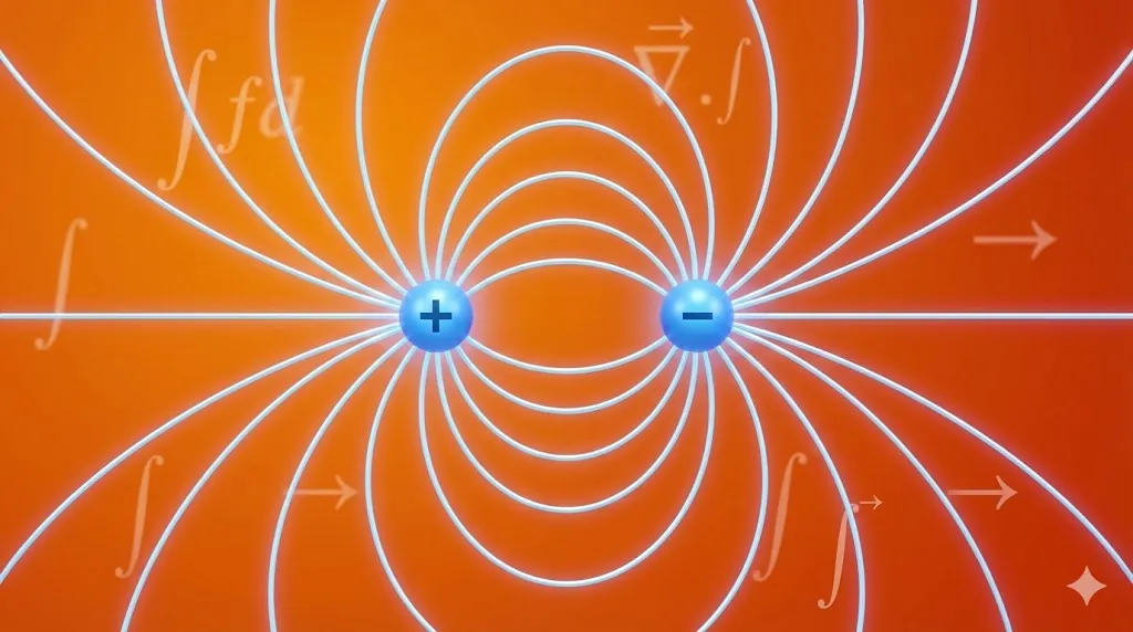
Properties of Electric Field Lines

Field line patterns for an isolated positive charge, an isolated negative charge, and an electric dipole. — Field lines originate on positive charges and terminate on negative charges.

Start on positive charge and end on negative charge.
Are continuous curves, with no breaks in charge-free region.
Never intersect: otherwise, field would have two directions at one point.
Do not form closed loops in electrostatics (field is conservative).

3. Electric Dipole Derivations

An electric dipole consists of charges $+q$ and $-q$ separated by distance $2a$ . Its dipole moment is $\vec{p} = q(2\vec{a})$ directed from negative to positive charge.

Derivation 1: Field on Axial Line 3 Marks

Geometry of a point P on the axis of a dipole, showing contributions from +q and -q. — Net field on the dipole axis is along the dipole moment.

Step 1: Expression for Fields Take point P at distance $r$ from the centre on axial line. Distances from charges are $r-a$ and $r+a$ .
$E_{+q} = \dfrac{kq}{(r-a)^2}, \quad E_{-q} = \dfrac{kq}{(r+a)^2}$

Step 2: Net Field Both fields are along the same direction (from $-q$ to $+q$ ):
$E_{net} = E_{+q} - E_{-q} = \dfrac{kq}{(r-a)^2} - \dfrac{kq}{(r+a)^2}$

Step 3: Simplify & Approximate Simplifying and using $p = 2qa$ , for $r \gg a$ :
$\vec{E}_{axial} = \dfrac{2\vec{p}}{4\pi\epsilon_0 r^3}$

Derivation 2: Field on Equatorial Line 3 Marks

Point P on perpendicular bisector of dipole, showing resolution of field vectors. — On the equatorial line, vertical components cancel, horizontal add opposite to $\vec{p}$ .

Step 1: Equal Magnitudes Distances from charges are equal. So $|E_{+q}| = |E_{-q}|$ .

Step 2: Components Vertical components cancel; horizontal components add opposite to dipole moment.

Step 3: Result for r ≫ a After substitution and approximation:
$\vec{E}_{eq} = -\dfrac{\vec{p}}{4\pi\epsilon_0 r^3}$

Derivation 3: Torque on Dipole in Uniform Field 2 Marks

Dipole at angle theta to uniform electric field showing forces +qE and -qE forming a couple. — Equal and opposite forces create a couple producing torque.

Concept In uniform field, net force is zero but forces $+qE$ and $-qE$ form a couple.

Torque Expression Perpendicular distance between forces is $2a\sin\theta$ .
$\tau = qE \cdot (2a \sin\theta) = pE \sin\theta$

Vector Form $\vec{\tau} = \vec{p} \times \vec{E}$

4. Continuous Charge Distribution

Charge Densities

Linear Density ( $\lambda$ ): Charge per unit length ( $\text{C/m}$ ).
Surface Density ( $\sigma$ ): Charge per unit area ( $\text{C/m}^2$ ).
Volume Density ( $\rho$ ): Charge per unit volume ( $\text{C/m}^3$ ).

5. Electric Flux & Gauss’s Law

Electric Flux Through Surface

\Delta\phi = \vec{E}\cdot\Delta\vec{S} = E\,\Delta S\,\cos\theta

Unit: N·m²/C

⚡

Gauss’s Law: The total electric flux through any closed surface is

\oint \vec{E} \cdot d\vec{S} = \frac{q_{in}}{\epsilon_0}

where $q_{in}$ is the net charge enclosed by the surface.

6. Applications of Gauss’s Law

Application 1: Infinite Straight Wire (Linear Charge Density $\lambda$ ) 5 Marks

Cylindrical Gaussian surface enclosing a section of an infinitely long charged wire. — By symmetry, field is radial and same over curved surface.

Gaussian Surface Choose a cylinder of radius $r$ and length $l$ coaxial with the wire. Enclosed charge: $q_{in} = \lambda l$ .

Flux Calculation Flux through circular ends is zero (field is radial). Only curved area $2\pi rl$ contributes: $\phi = E (2\pi rl)$ .

Final Result Apply Gauss’s law: $E (2\pi rl) = \dfrac{\lambda l}{\epsilon_0} \Rightarrow$
$E = \dfrac{\lambda}{2\pi\epsilon_0 r}$

Application 2: Infinite Plane Sheet (Surface Density $\sigma$ ) 5 Marks

Gaussian pillbox piercing through an infinite plane sheet of charge. — Flux passes only through the flat faces of the pillbox.

Gaussian Surface Take a thin pillbox of cross-sectional area $A$ cutting the sheet. Enclosed charge: $q_{in} = \sigma A$ .

Flux Calculation Field is perpendicular to sheet on both sides: total flux $\phi = EA + EA = 2EA$ .

Final Result Using Gauss’s law: $2EA = \dfrac{\sigma A}{\epsilon_0} \Rightarrow$
$E = \dfrac{\sigma}{2\epsilon_0}$ (independent of distance $r$ ).

Application 3: Thin Spherical Shell (Total Charge $q$ ) 5 Marks

Gaussian sphere outside and inside a uniformly charged spherical shell. — The shell behaves like a point charge from outside and has zero field inside.

Case A: Outside the Shell ( $r > R$ ) Gaussian sphere radius $r$ encloses charge $q$ .
From symmetry, $E$ is radial and constant over surface: $E(4\pi r^2) = \dfrac{q}{\epsilon_0} \Rightarrow$
$E = \dfrac{q}{4\pi\epsilon_0 r^2}$

Case B: Inside the Shell ( $r < R$ ) Gaussian sphere encloses no charge: $q_{in} = 0$ . Hence
$E = 0$ everywhere inside the hollow shell.

← Unit Dashboard Next Chapter: Potential & Capacitance →